Implementation Report: Predict Function
1 Introduction
This report provides an overview of the proposed predict() function’s implementation in DIPY’s Generalized Q-Sampling Imaging (GQI) model, including the newly implemented prediction_kernel() and the pre-existing gqi_kernel() helper functions.
It covers their purpose, operational mechanics, mathematical foundations, testing methodology, and obtained results.
2 The Different Needed Helper Functions
The predict() function implementation relies on two key helper functions:
gqi_kernel()(pre-existing) for kernel computationprediction_kernel()(newly implemented) for pseudo-inverse calculation.
In this section, each function is described in detail, including its purpose, parameters, and role in signal reconstruction from ODFs.
2.1 The gqi_kernel() Function
The gqi_kernel() function calculates the Generalized Q-Sampling Imaging (GQI) transformation kernel, which is essential for modeling diffusion signals in terms of orientation distribution functions (ODFs). This kernel transforms gradient directions and b-values into a matrix that relates diffusion signals to ODFs on a spherical grid.
- Purpose: Computes the kernel matrix for GQI-based signal reconstruction. It handles different GQI methods (
standardorgqi2) and incorporates physical constants like the free water diffusion coefficient. - Key Parameters:
gtab: GradientTable containing b-values and b-vectors.param_lambda: Regularization parameter for the kernel.sphere: Spherical grid for ODF sampling.method: Specifies the GQI variant (standardby default).
- Operation: Scales b-vectors by a diffusion-related factor, computes dot products with sphere vertices, and applies sinc or squared radial functions to generate the kernel.
def gqi_kernel(gtab, param_lambda, sphere, method="standard"):
    # 0.01506 = 6*D where D is the free water diffusion coefficient
    # l_values sqrt(6 D tau) D free water diffusion coefficient and
    # tau included in the b-value
    scaling = np.sqrt(gtab.bvals * 0.01506)
    b_vector = gtab.bvecs * scaling[:, None]

    if method == "gqi2":
        H = squared_radial_component
        return np.real(H(np.dot(b_vector, sphere.vertices.T) * param_lambda))
    elif method != "standard":
        warnings.warn(
            f'GQI model "{method}" unknown, falling back to "standard".',
            stacklevel=1,
        )
    return np.real(np.sinc(np.dot(b_vector, sphere.vertices.T) * param_lambda / np.pi))
Mathematically, the GQI kernel \(K\) is computed as:
For the standard method: \[
K_{ij} = \frac{\sin\left( \lambda (\mathbf{q}_i \cdot \mathbf{v}_j) \right)}{\lambda (\mathbf{q}_i \cdot \mathbf{v}_j)} = \operatorname{sinc}\left( \frac{\lambda (\mathbf{q}_i \cdot \mathbf{v}_j)}{\pi} \right)
\] Where:
- \(\mathbf{q}_i = \mathbf{g}_i \sqrt{b_i \cdot 0.01506}\) (scaled gradient)
- \(\mathbf{v}_j\) are sphere vertices
- \(\lambda\) is the regularization parameter
- \(\operatorname{sinc}(x) = \frac{\sin(\pi x)}{\pi x}\) is the NumPy’s normalized
sinc()function.
For the gqi2 method: \[
K_{ij} = \operatorname{Re}\left[ H\left( \lambda (\mathbf{q}_i \cdot \mathbf{v}_j) \right) \right]
\] Where \(H\) is the squared radial component function (see eq.8 in the referenced paper Yeh, Wedeen, and Tseng 2010)
2.2 The prediction_kernel() Function
The prediction_kernel() function computes the Tikhonov-regularized Moore-Penrose pseudo-inverse of the GQI kernel, enabling signal reconstruction from orientation distribution functions (ODFs) in the DIPY convention.
- Purpose: Generates the Tikhonov-regularized pseudo-inverse kernel for solving S from \(ODF = S \cdot K\), using regularization for numerical stability.
- Key Parameters:
gtab: GradientTable for the prediction.param_lambda:gqi_kernelregularization parameter.sphere: Spherical grid.method: GQI method.
- Operation: Computes the GQI kernel \(K\), forms \(K \cdot K^{T}\), adds regularization, inverts the matrix, and multiplies by \(K^{T}\) to produce the Tikhonov-regularized Moore-Penrose pseudo-inverse kernel.
INVERSE_LAMBDA = 1e-6

def prediction_kernel(gtab, param_lambda, sphere, method="standard"):
    # K.shape = (n_gradients, n_vertices)
    K = gqi_kernel(gtab, param_lambda, sphere, method=method)

    # GTG.shape = (n_gradients, n_gradients)
    GtG = K @ K.T
    identity = np.eye(GtG.shape[0])

    # K_plus.shape = (n_vertices, n_gradients)
    return K.T @ np.linalg.inv(GtG + INVERSE_LAMBDA * identity)
Mathematically, the prediction kernel \(K^{+}\) is computed as: \[ K^{+} = K^T (K K^T + \lambda I)^{-1} \] Where:
- \(K\) is the GQI kernel from
gqi_kernel() - \(\lambda\) is the regularization parameter (
INVERSE_LAMBDA) - \(I\) is the identity matrix.
The Tikhonov regularization term (\(\lambda I\)) is added to improve numerical stability and prevent overfitting. The plain Moore-Penrose pseudo-inverse, computed as \(K^T (K K^T)^{-1}\), can be unstable for ill-conditioned matrices, amplifying noise in the diffusion signals. Regularization provides a smoother, more robust solution by balancing fidelity to the data with stability.
3 The predict() Function And Its Implementation
The target predicted signal is given by the following relationship \[ \begin{alignat*}{2} &ODF &&= S \cdot K \\ \iff\quad & ODF \cdot K^{+} &&\approx S \cdot K \cdot K^{+} \\ \iff\quad & ODF \cdot K^{+} &&\approx S \\ \iff\quad & S &&\approx ODF \cdot K^{+} \end{alignat*} \]
Where:
- \(S\) is the GQI model fitted signal
- \(K^{+}\) is the Tikhonov-regularised Moore-Penrose pseudo-inverse of the GQI kernel \(K\).
Note that the pseudo-inverse is needed since the GQI kernel \(K\)’s dimensions are \((n_\mathrm{gradients}, n_\mathrm{vertices})\), which means it’s (most of the time) not a square matrix and therefore does not have a true inverse.
The predict() function reconstructs diffusion signals from the fitted signal data by fusing the model kernel and the pseudo-inverse kernel to avoid explicit ODF computation.
- Purpose: Predicts diffusion-weighted signals from fitted data, supporting both single-voxel and multi-voxel data.
- Key Parameters:
gtab: GradientTable for which to predict signals.S0: Optional baseline signal (not used in this implementation).
- Operation: Fuses the model kernel and prediction kernel to avoid explicit \(ODF\) computation:
combined_kernel= \(K_\mathrm{model}^T \cdot K^+\), thenpredicted = data @ combined_kernel. Handles data reshaping for matrix operations and ensures non-negative outputs by clamping values.
def predict(self, gtab, *, S0=None):
    # K_plus.shape = (n_vertices, n_gradients)
    K_plus = prediction_kernel(
        gtab,
        self.model.Lambda,
        self.model.sphere,
        self.model.method,
    )

    # Fuse kernel and prediction kernel to avoid explicit ODF computation:
    # combined_kernel.shape = (n_gradients_original, n_gradients)
    combined_kernel = self.model.kernel.T @ K_plus

    # Handle both 1D (single voxel) and multi-dimensional data
    if self.data.ndim == 1:
        # Single voxel: data = (self.model.n_gradients,)

        # predicted.shape = (n_gradients, )
        predicted = self.data @ combined_kernel
    else:
        # Multi-voxel: data = (..., self.model.n_gradients)
        original_shape = self.data.shape
        data_2d = self.data.reshape(-1, original_shape[-1])

        # predicted_2d.shape = (n_voxels, n_gradients)
        predicted_2d = data_2d @ combined_kernel

        # predicted.shape = (..., n_gradients)
        predicted = predicted_2d.reshape(
            original_shape[:-1] + (combined_kernel.shape[1],)
        )

    # Clamp to non-negative values
    return np.maximum(predicted, 0)
Mathematically, the predicted signal \(\mathbf{S}_\mathrm{pred}\) is computed as: \[ \mathbf{S}_\mathrm{pred} = \max(0, \mathrm{ODF} \cdot K^{+}) \] Where:
- \(\mathrm{ODF} = K_\mathrm{model} \cdot \mathbf{S}_\mathrm{data}\) is the ODF computed from the fitted signal data
- \(K^{+}\) is the pseudo-inverse kernel from
prediction_kernel()
Equivalently, this can be computed directly as \(\mathbf{S}_\mathrm{pred} = \max(0, \mathbf{S}_\mathrm{data} \cdot (K_\mathrm{model}^T \cdot K^{+}))\) to avoid intermediate ODF calculation for efficiency.
The \(\max\) operation ensures non-negative signal values.
4 Testing Methodology
The testing methodology for the GQI prediction functions encompasses unit tests for individual components and integration tests for end-to-end prediction workflows.
These tests validate:
- mathematical correctness
- numerical stability
- practical usability across single and multi-voxel scenarios.
All tests utilize DIPY’s small_101D dataset1 and simulated diffusion MRI datasets with known properties to ensure robustness.
4.1 prediction_kernel() Function Tests
The prediction_kernel() function is tested for its role as a Tikhonov-regularized Moore-Penrose pseudo-inverse of the GQI kernel. Key validations include:
- Shape and finiteness: Ensures the kernel has correct dimensions \((n_\mathrm{vertices}, n_\mathrm{gradients})\) and contains only finite values, with at least one non-zero value.
- Pseudo-inverse properties: Verifies that \(K K^+ K \approx K\) (regularized reconstruction), and that \(K K^+\) and \(K^+ K\) are symmetric matrices.
- Method compatibility: Tests both
standardandgqi2GQI methods using thesymmetric724sphere and DSI gradient table.
These tests confirm the kernel’s mathematical integrity and numerical stability for signal reconstruction.
4.2 Basic API predict() Function Tests
Basic prediction tests validate the predict() function’s API and output characteristics for both single-voxel and multi-voxel data:
- Single-voxel test: Fit the model to individual voxels from DSI data, predict signals, and check that outputs are non-negative arrays matching the gradient table length. It also includes predictions on subsets of gradients.
- Multi-voxel test: Fit the model to entire 3D volumes, predict signals, and verify shape preservation and non-negativity. Subset gradient predictions are also tested.
- Method coverage: Both
standardandgqi2methods are tested to ensure consistent behavior.
These tests ensure the prediction function handles various data shapes and gradient configurations correctly.
4.3 Round Trip predict() Function Tests
Round-trip tests assess the fidelity of signal reconstruction by fitting the model to training data (excluding b0 volumes) and predicting back to the same gradient table.
These tests are performed exclusively on the standard GQI model. Correlation between original and predicted signals serves as a quality metric.
- Single-voxel round-trip: For selected voxels, compute Pearson correlation between original and predicted signals. Assert correlations exceed \(r > 0.8\) and signal magnitudes remain in the same order of magnitude.
- Multi-voxel round-trip: Compute average correlation across all voxels in the volume, requiring \(\bar{r} > 0.8\). Identify and reject any voxels with \(r \leq 0.8\).
These tests quantify reconstruction accuracy and detect underfitting or numerical instabilities.
5 Obtained Results
Building on the testing methodology outlined above, the obtained results validate the implementation using real DSI data from the DIPY library. They demonstrate high accuracy in signal reconstruction and generalization, quantified by voxel-wise correlation metrics and visual comparisons against ground truth data.
In the following subsections, we present the results for single-voxel and multi-voxel roundtrip predictions, followed by generalization to unseen data.
5.1 Single-Voxel Reconstruction Results
Results from the single-voxel roundtrip test on the small_101D dataset are presented here, focusing on signal reconstruction for a representative voxel.
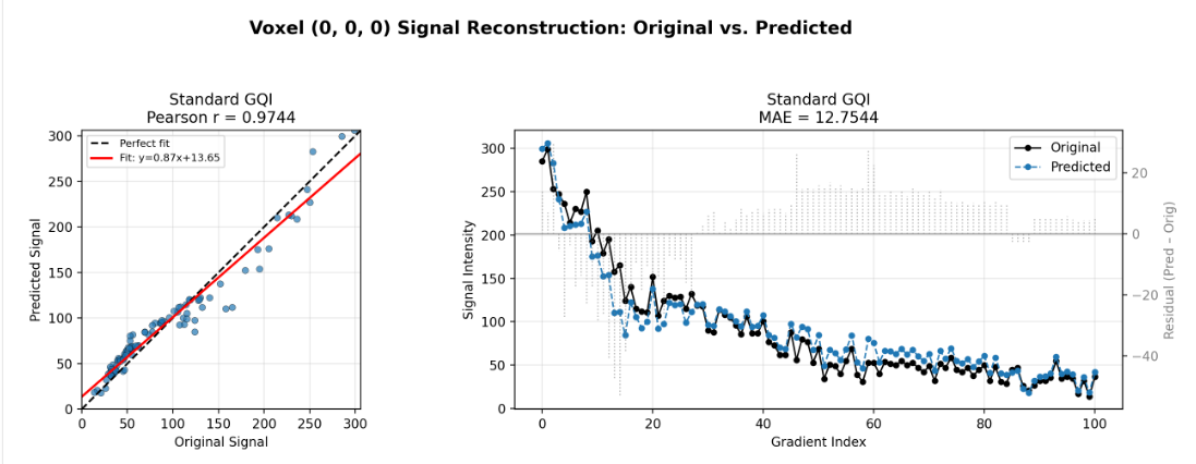
The plots in Figure 1 provide a detailed analysis for a single representative voxel.
- Strong Linear Relationship: The scatter plot on the left shows a strong positive linear relationship between the original and predicted signals, with a Pearson correlation coefficient of \(r = 0.9744\). The fitted line \(y = 0.87x + 13.65\) closely tracks the identity line (dashed black), indicating minimal bias in the prediction.
- Signal Profile Fidelity: The line plot on the right compares the signal intensity profiles across all gradient directions. The predicted signal (in blue) closely follows the original signal (in black). The residual plot (in gray) shows small deviations, with an \(MAE\) of \(12.7544\), which is acceptable given the signal range (~0-300).
These results demonstrate the effectiveness of the predict() function for single-voxel predictions.
For the complete single-voxel roundtrip analysis, refer to the GQI Roundtrip notebook.
5.2 Multi-Voxel Reconstruction Results
The multi-voxel roundtrip test on the small_101D dataset evaluates reconstruction accuracy across the entire volume, with results shown below.
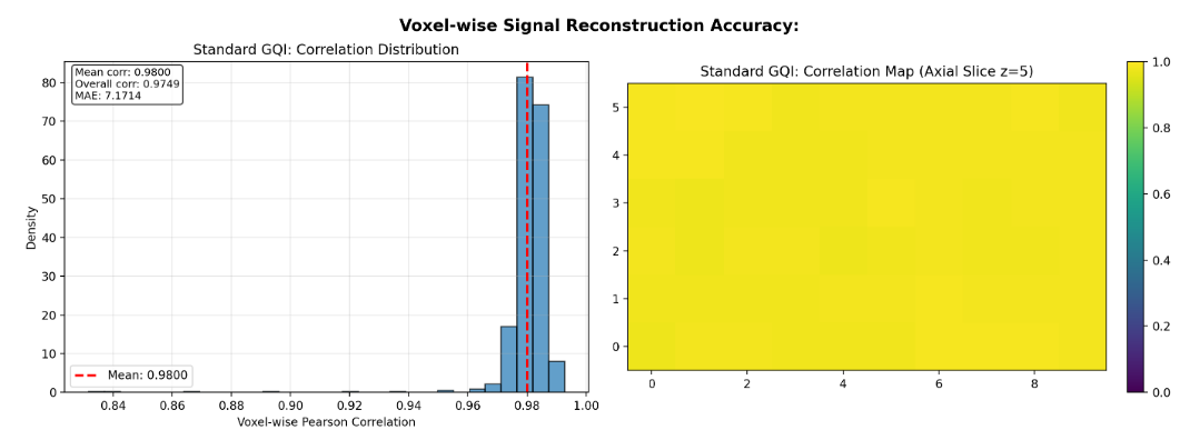
The histogram presented in Figure 2 shows the distribution of Pearson correlation coefficients between original and predicted signals across all voxels for the “Standard GQI” model.
- High Overall Fidelity: The distribution is sharply peaked near perfect correlation (\(r=1.0\)), indicating the model successfully reconstructs the training data.
- Quantitative Metrics: The mean voxel-wise correlation is \(0.9800\), and the overall correlation across the entire volume is \(0.9749\), both significantly exceeding the target thresholds of \(r > 0.8\) and \(\bar{r}>0.8\). The \(MAE\) of \(7.1714\) further confirms low prediction error relative to the signal intensity scale.
- Spatial Consistency: The accompanying correlation map (right panel) shows a uniformly high correlation (yellow tones) across the middle slice, confirming that the model’s performance is spatially consistent and not localized to specific regions.
This validates the numerical stability and robustness of the predict() function for multi-voxel data.
See the GQI Roundtrip notebook for detailed multi-voxel implementation.
5.3 Prediction On Unseen Data
To illustrate generalization, this section shows predictions for unseen gradient configurations using the taiwan_ntu_dsi dataset2
The model was fitted on existing gradients and is used to predict signals for an unseen gradient (unseen b-value and b-vector).
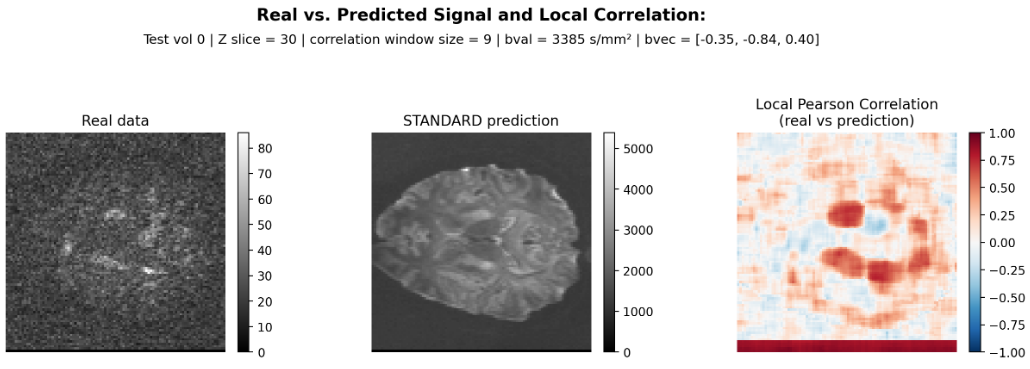
The visualization in Figure 3 evaluates the model’s ability to generalize to unseen gradient configurations.
- Visual Agreement: A side-by-side comparison of the
Real dataandstandard predictionfor a specific b-value and b-vector shows a strong qualitative match. The predicted image successfully captures the anatomical structure and intensity variations present in the real data, including bright white matter tracts. - Local Correlation Validation: The Local Pearson Correlation map, computed over a 9x9 window, quantifies this agreement. The map displays predominantly red and orange regions (correlation > 0.5), indicating good local correspondence between the real and predicted signals. While some areas show lower correlation (blue/purple), these are likely associated with complex fiber crossings or noise, which is expected in diffusion MRI.
This demonstrates the model’s capability to predict signals for new, unseen gradients beyond the training set.
The full unseen prediction workflow is available in the GQI Unseen Data notebook.
These results collectively confirm that the implemented predict() function is mathematically sound, numerically stable, and practically effective for both reconstructing training data and generalizing to new gradient directions. The high correlation values and visual fidelity validate the correctness of the Tikhonov-regularized pseudo-inverse approach used in the prediction_kernel() function.
6 Conclusion
In summary, the implementation of the predict() function for DIPY’s GQI model has been successfully validated through comprehensive testing on real DSI datasets. The function accurately reconstructs diffusion signals for both single-voxel and multi-voxel scenarios, as evidenced by high correlation coefficients and low mean absolute errors in roundtrip tests.
Furthermore, it demonstrates strong generalization capabilities to unseen gradient configurations, confirming its practical utility in diffusion MRI analysis. The Tikhonov-regularized pseudo-inverse approach ensures numerical stability and robustness, providing a reliable tool for signal prediction in advanced neuroimaging workflows.
7 Extra Resources
This section contains extra resources to go deeper into the topics covered in this report.
7.1 DIPY Tutorial Notebooks
These notebooks were created based off the DIPY documentation examples for this project.
7.2 Project-Specific Notebooks
These notebooks were developed specifically for this project to demonstrate the predict() function implementation, validation, and application.