CBI Presentation

Olivier Amacker

2026-07-24

What Is The Problem With The Current fMRI Pipelines?

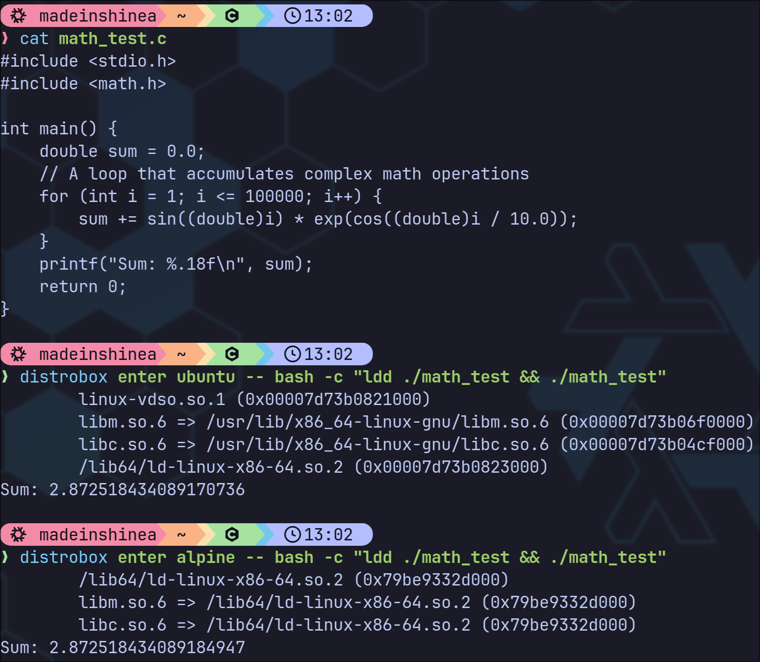
Currently the fMRI pipelines are becoming more and more computationally heavy leveraging a lot of high dimension calculations.

However, there are several settings introducing noise instability in those pipelines:

• The OS running the pipeline and its version
• The actual hardware (CPU architecture)
• Parallelization strategies

Figure 1: Example of the same program giving different results depending on the OS

What Can We Do About It?

We can artificially introduce numerical perturbations inside the floating point arithmetic with the help of tools like Verificarlo(Denis, Castro, and Petit (2018)) and Fuzzy and assess how the desired pipeline’s results change to make sure it is stable.

Verificarlo is a compiler wrapper that instruments floating point operations at the LLVM level.

Fuzzy is a Docker ecosystem that provides pre instrumented versions of common numerical libraries so you can evaluate a pipeline’s stability without recompiling your own code.

Was This Done Before?

Yes, there are already several papers on the subject, like Alizadeh et al. (2026) or Chatelain et al. (2026).

But numerical instability is not transferable across pipelines, it comes from each pipeline’s specific algorithms, operation orders, software stacks etc.

Benchmarking each one is essential.

What Did I Do Regarding that?

My job was to look into the numerical stability of fMRI biomarkers.

To do so, I focused on three main tasks:

• Reproduce the Alizadeh et al. (2026) paper on NPVR of MRI graph metrics
• Perturb fMRIPrep (Esteban et al. (2019)) runs via Verificarlo and assess changes in FC matrices
• Assess whether the Yamashita et al. (2026) PCA feature selection remains stable under numerical perturbations

A detailed summary of what I did each day is available here

Figure 2: daily journal QR code

Alizadeh et al. (2026) Paper Goals

The paper has two goals:

• Demonstrate on artificial data that NPVR increase uncertainty in Cohen’s \(d\) estimates, with stronger effects at small \(n\).
• Assess how numerical perturbations via Verificarlo of fMRIPrep runs impact the NPVR of various graph metrics.

Here is the formula for the NPVR:

\[NPVR = \frac{\sigma_{num}}{\sigma_{pop}}\]

Where \(\sigma_{num}\) is the numerical variability and \(\sigma_{pop}\) is the population variability.

Alizadeh et al. (2026) Reproduction Resources

A summary of this paper is available here

Figure 3: Alizadeh et al. (2026) paper summary QR code

The code used for this section is available here

Figure 4: NPVR notebook QR code

Artificial NPVR Results Comparison

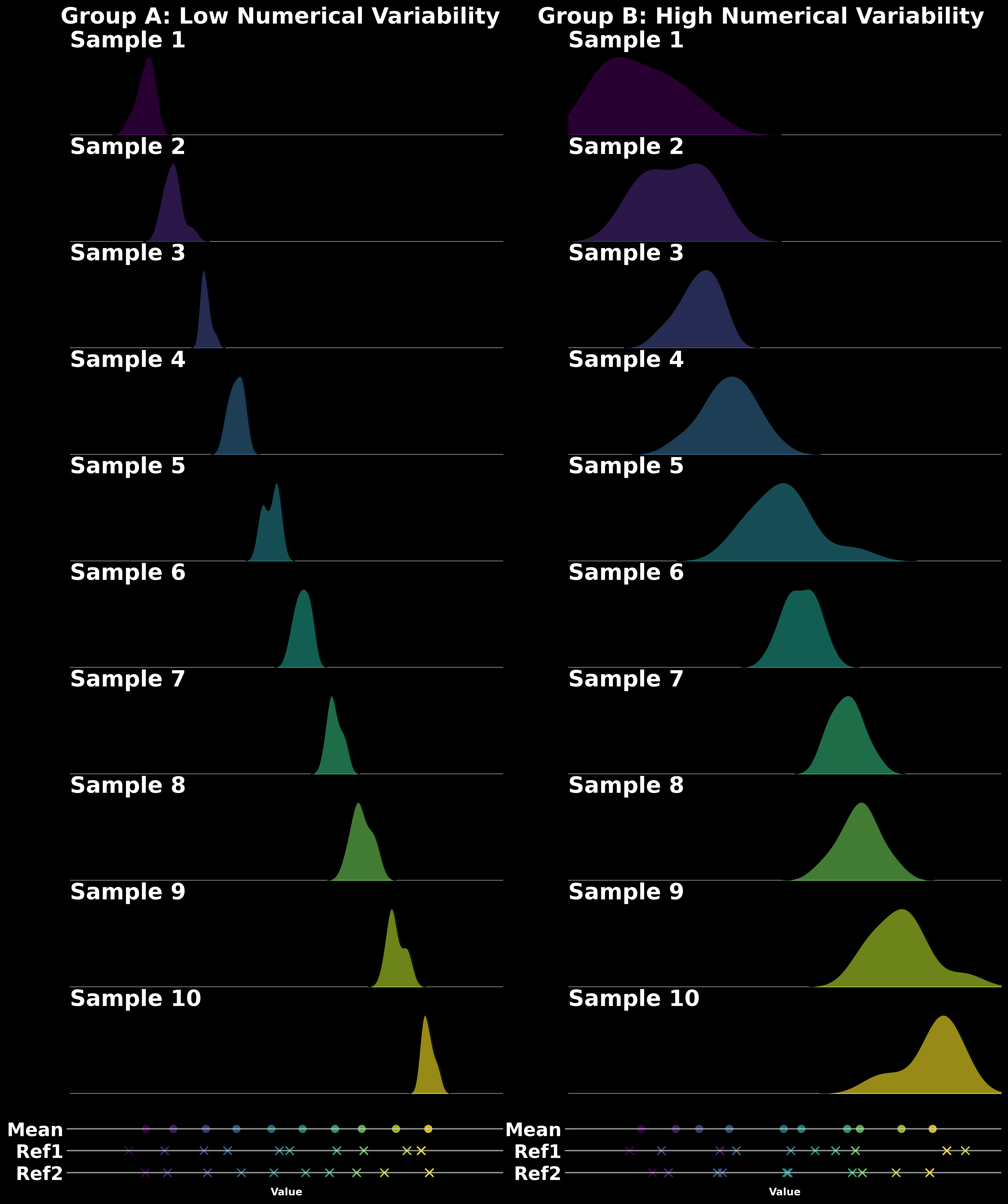
Figure 5: Population distribution (mine)

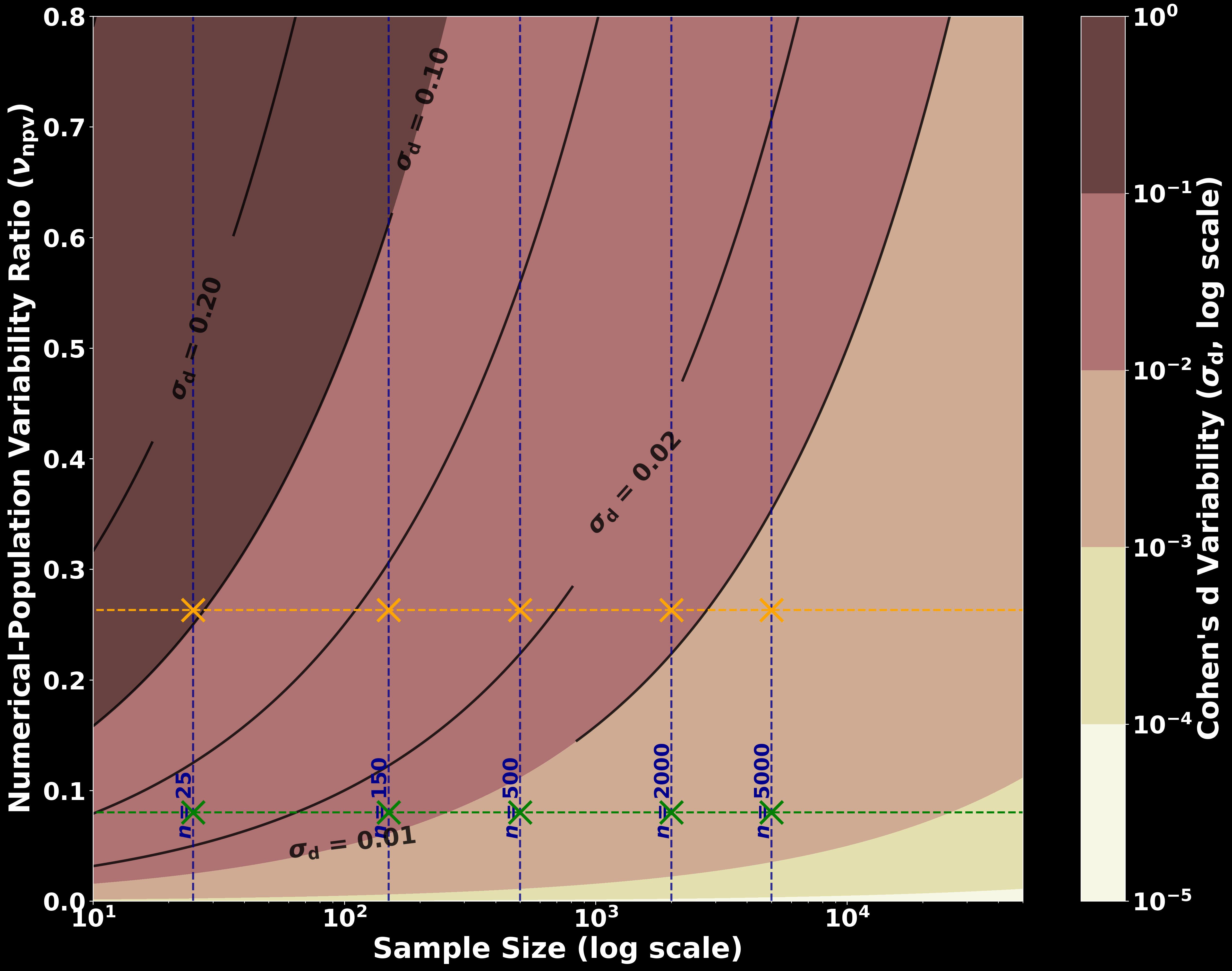
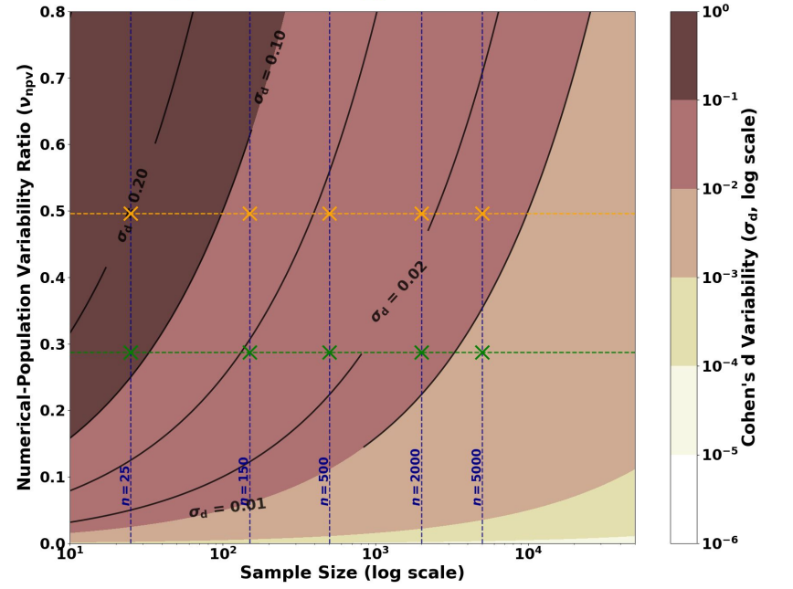
Figure 6: Relation between the NPVR and the Cohen’s \(d\) (mine)

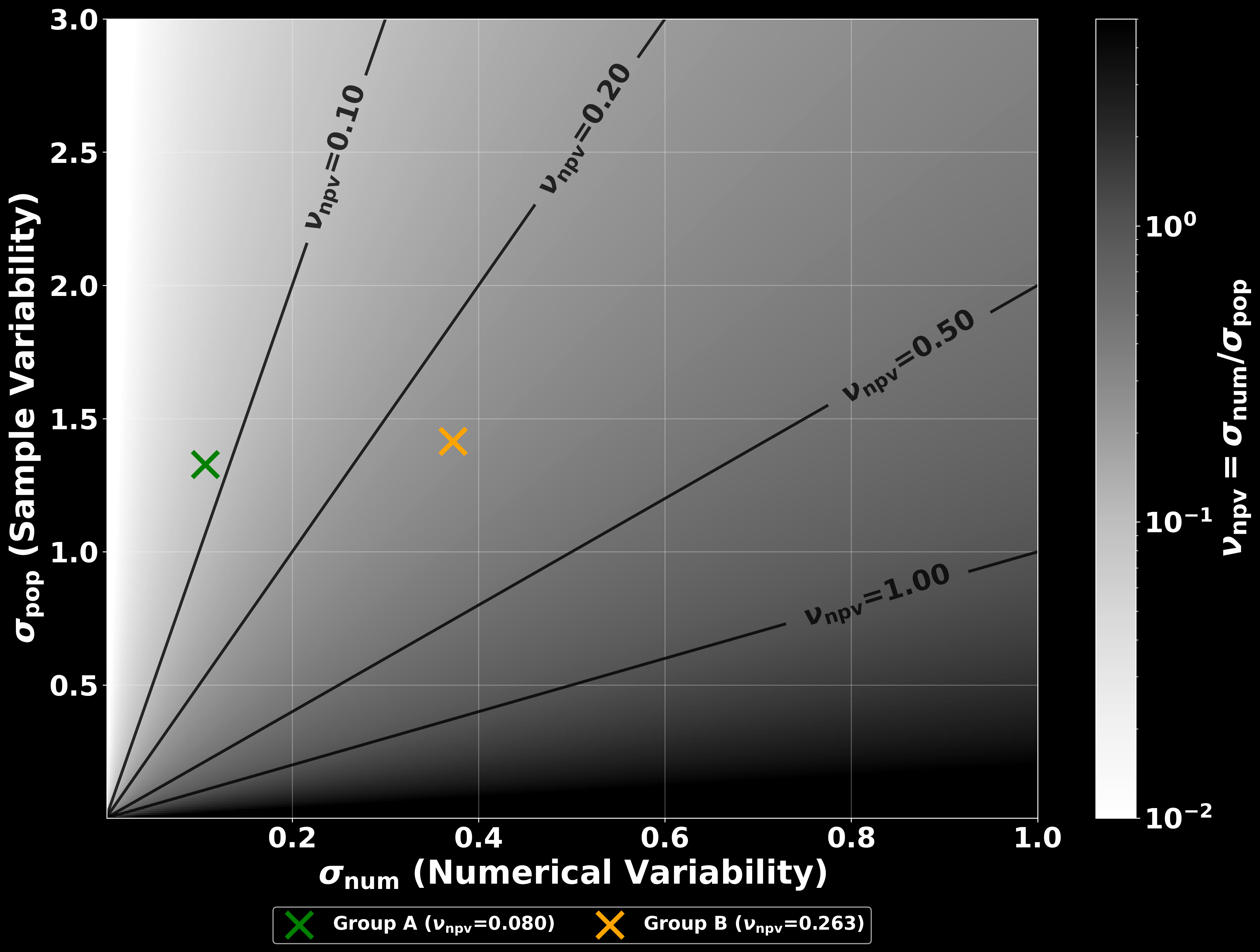
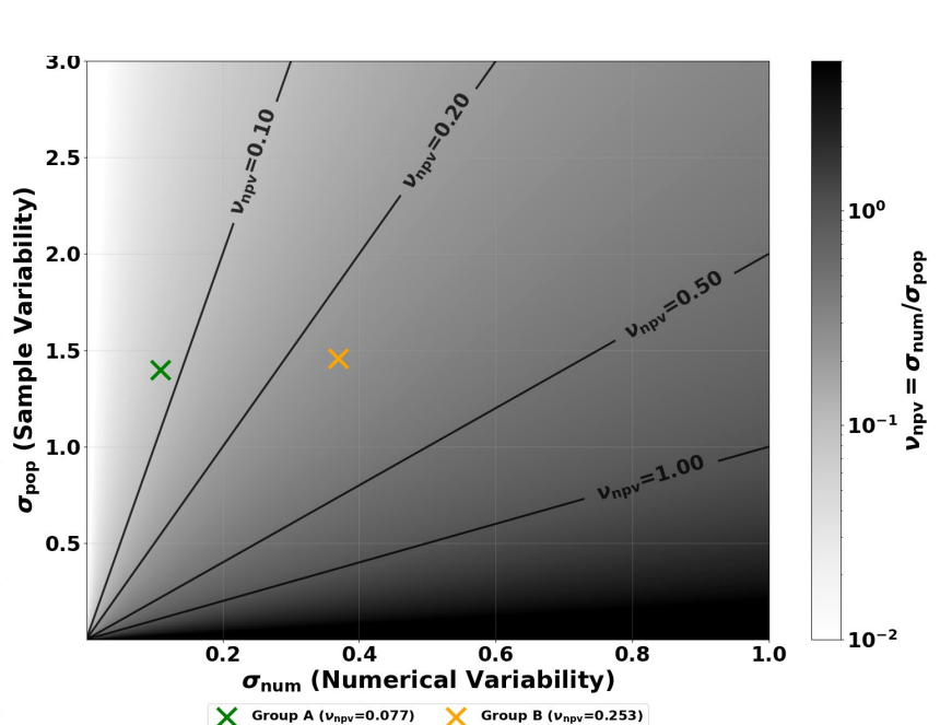
Figure 7: Relation between pop and num var (mine)

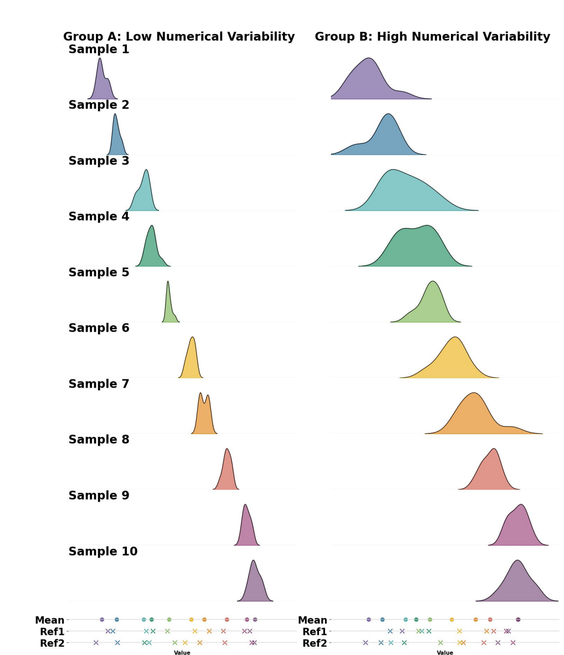
Figure 8: Population distribution (paper)

Figure 9: Relation between the NPVR and the Cohen’s \(d\) (paper)

Figure 10: Relation between pop and num var (paper)

Artificial NPVR PR

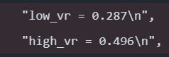
Regarding the Relation between the NPVR and the Cohen’s \(d\) differences, a PR was opened and merged into the paper’s repository (see here)

Figure 11: Hard coded values for the 2nd graph

Alizadeh et al. (2026) Graph Metrics

Here are the different graph metrics that were computed once with and once without confounds regression

Four local graph metrics were computed:

• Degree centrality
• Clustering coefficient
• Betweenness centrality
• Eigenvector centrality

Two global metrics:

• Small-worldness
• Average shortest path length

Graph Metrics Reproduction Code

The code used for this section is available here

Figure 12: Graph Metrics notebook QR code

Graph Metrics Results Comparison

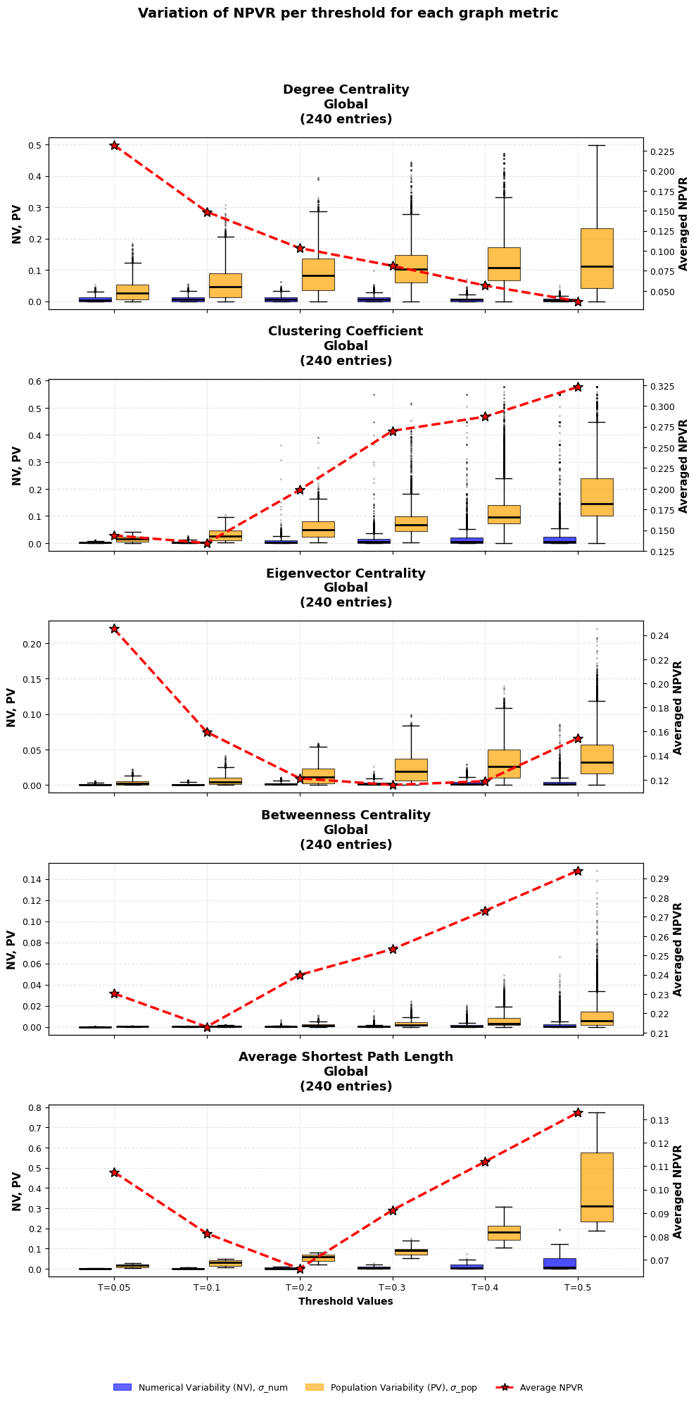
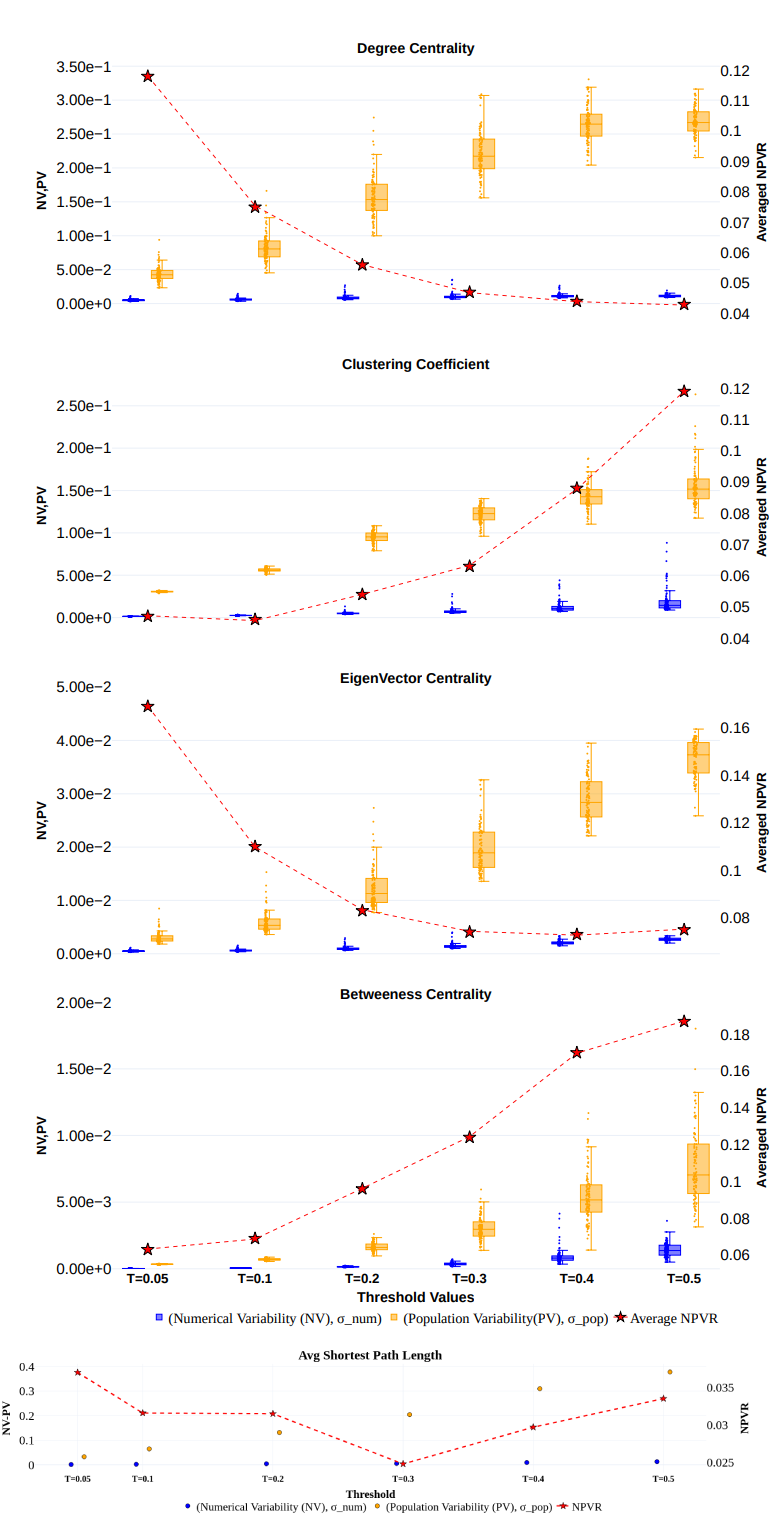
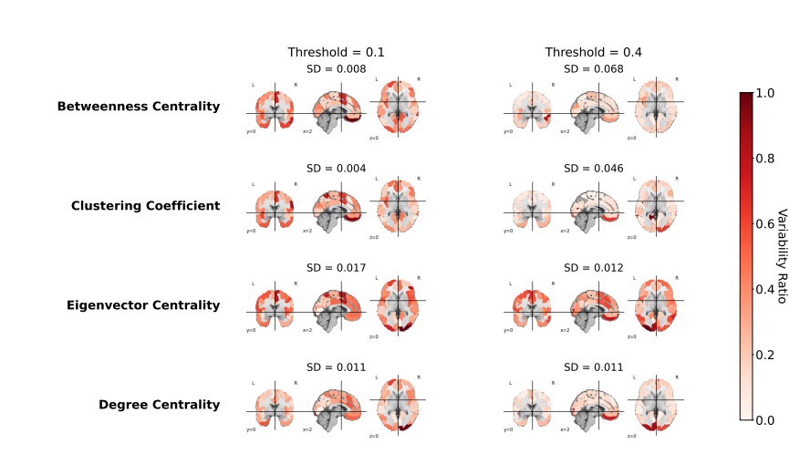
Figure 13: Graph metrics NPVR per threshold (mine)

Figure 14: Graph metrics NPVR per threshold (paper)

Graph Metrics Results Comparison

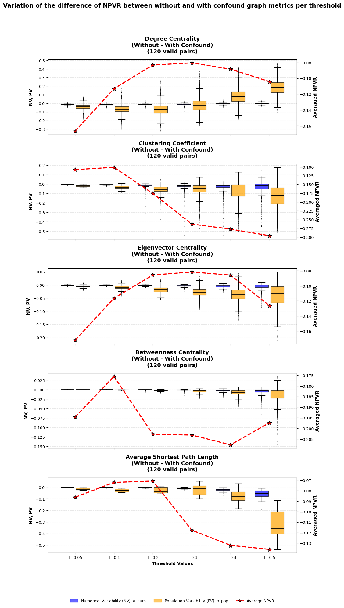
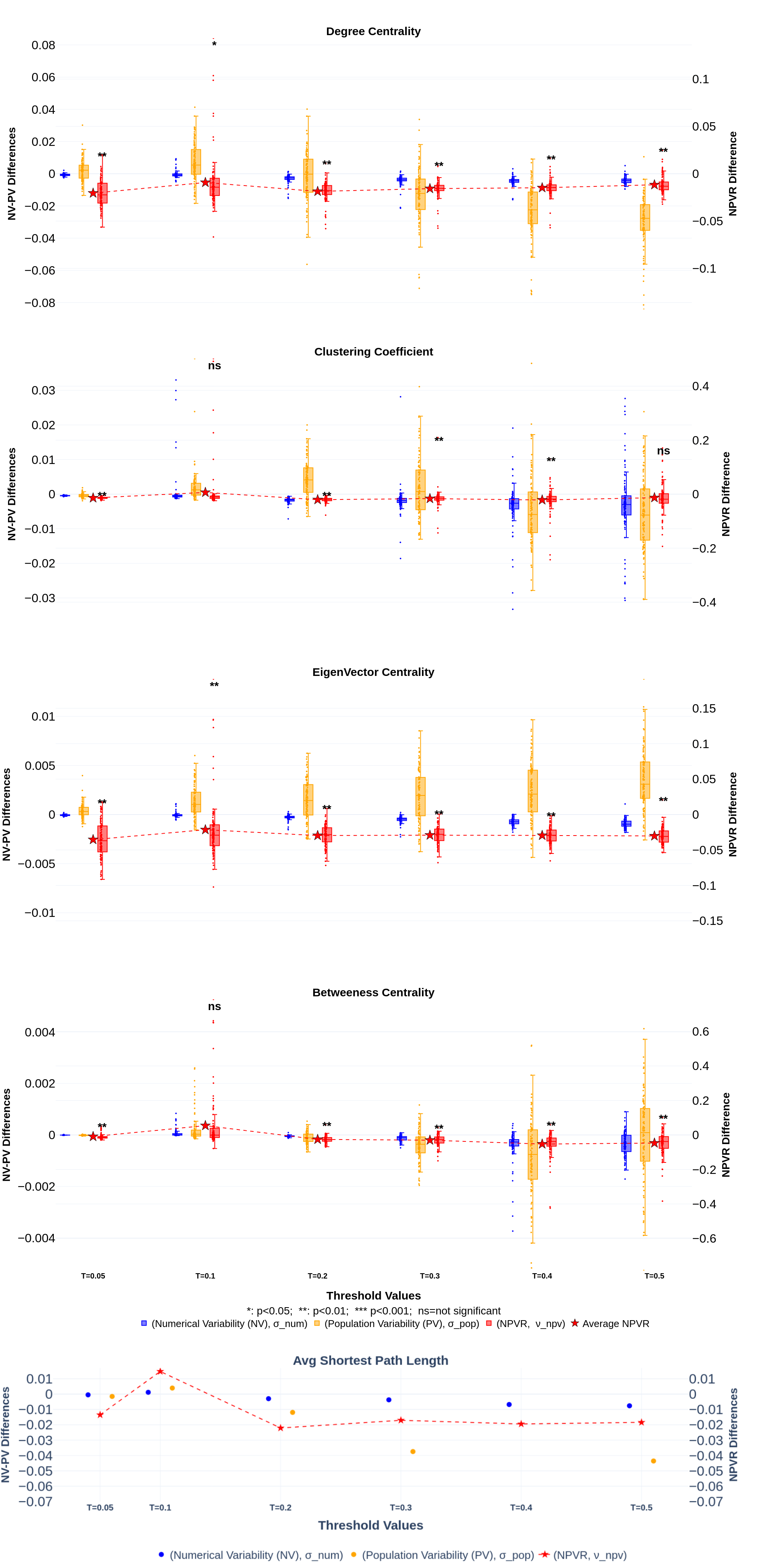
Figure 15: Variation of the NPVR between without and with confound (mine)

Figure 16: Variation of the NPVR between without and with confound (paper)

Graph Metrics Results Comparison

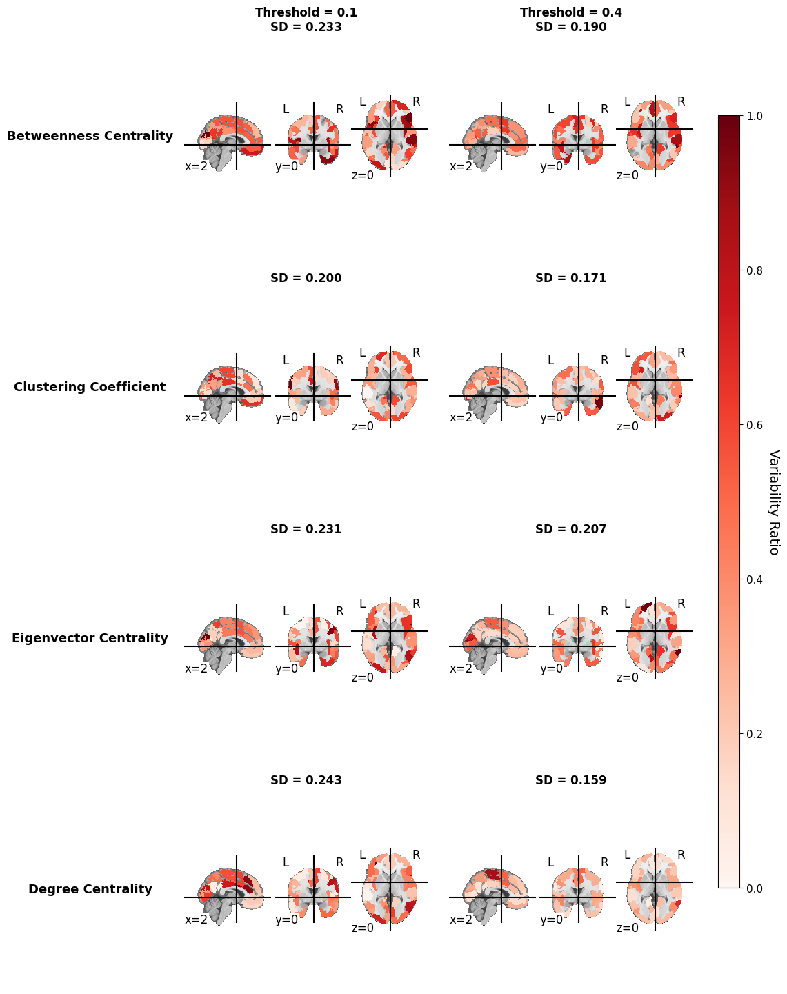
Figure 17: Degree centrality NPVR values across brain regions and thresholds (mine)

Figure 18: NPVR values across brain regions and thresholds (paper)

Perturbed fMRIPrep Runs FC Matrices Analysis Goals

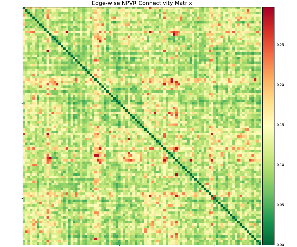
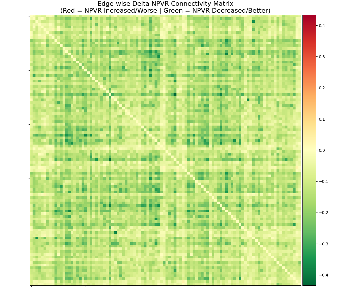
The goal of this section was to take the numerically perturbed fMRIPrep runs that were made so far, and assess how the NPVR changes across the different FC matrix edges.

So this looks into the FC matrices directly rather than graph metrics like the previous section.

Perturbed fMRIPrep Runs FC Matrices Analysis Code

The code used for this section is available here

Figure 19: Fuzzy FC matrices notebook QR code

Perturbed fMRIPrep Runs FC Matrices Analysis Results

Figure 20: NPVR across FC matrix edges with all the confounds regressions

Figure 21: NPVR across FC matrix edges difference between with and without the global confound regression

Yamashita et al. (2026) PCA Feature Selection Stability Analysis

The goal of this paper is to develop a PCA-based feature selection method that robustly extracts reliable FC biomarkers for major depressive disorder (MDD), schizophrenia (SCZ), and autism spectrum disorder (ASD) across multiple independent datasets and imaging sites, overcoming the instability issues of conventional supervised feature selection approaches.

Original PCA Feature Selection Explanation

The PCA feature selection works as follows:

• A PCA is computed on all subjects’ FC vector to reduce dimensionality to n principal components.
• PCs are tested for association with variables of interest:
  • Binary categorical (e.g., diagnosis, sex): two-sample t-test
  • Multi-level categorical (e.g., imaging site): one-way ANOVA
  • Continuous (e.g., age, BDI, head motion): Pearson’s correlation
• Select PCs significantly associated with the target after FDR-BH correction (q < 0.05)
• Test FC weights using a chi-squared test with FDR-BH correction (q < 0.05)
• Keep only FCs that survive the correction as the final biomarkers

What Did I Change In The PCA Feature Selection Code?

I made several changes to the PCA feature selection code:

• Transformed the repository from regular Python code to a Python package (see PR here)
• Improved the PC plots (see PR here)
• Added a more stable option for the PC selection (see PR here)

PCA Feature Selection Stability Analysis Code

The code used for this section is available here

Figure 22: Fuzzy PCA analysis notebook QR code

PCA Feature Selection Stability Analysis Procedure

To conduct this analysis, I performed the following steps:

• Reproduced the PCA feature selection on the complete SRPB dataset (which was split into training and test sets)
• Reproduced the PCA feature selection on the BMB dataset (a new dataset)
• Ran 100 perturbated runs of the SRPB dataset FC matrix extraction (perturbing the np.corrcoef function)
• Ran 15 perturbated runs of the BMB dataset FC matrix extraction

The PCA feature selection was performed on each of the perturbated runs

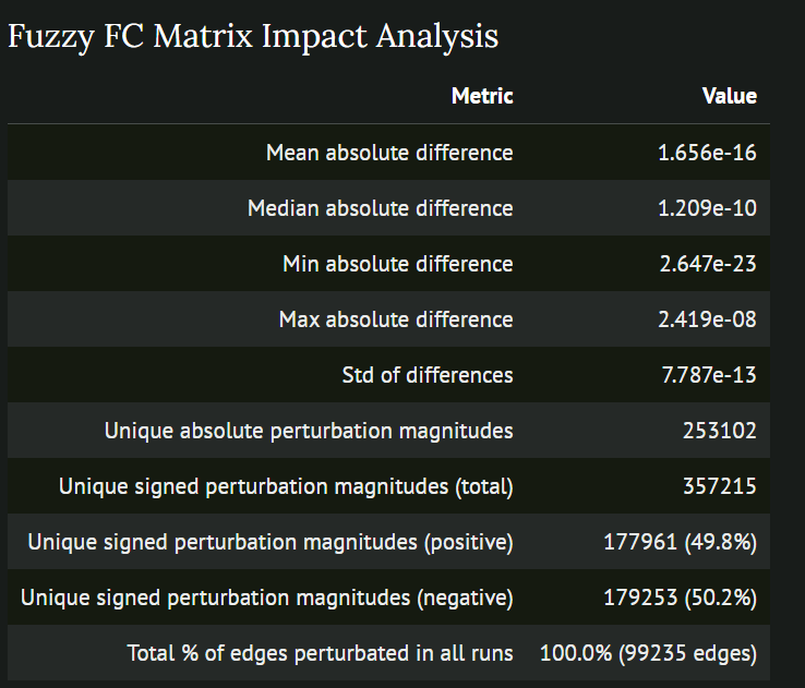
What was the effect of the np.corrcoef perturbation?

Effect of the np.corrcoef perturbation on \(\text{16 542 474 500}\) edges

PCA Feature Selection Stability Results

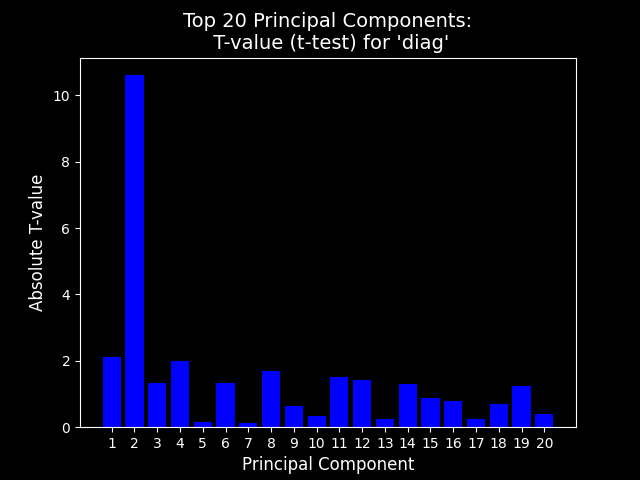
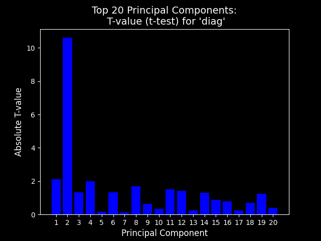
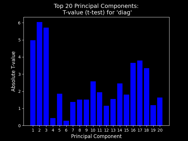
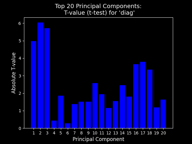
Figure 23: SRPB fuzzy run 0 diagnostic PC plot

Figure 24: SRPB original diagnostic PC plot

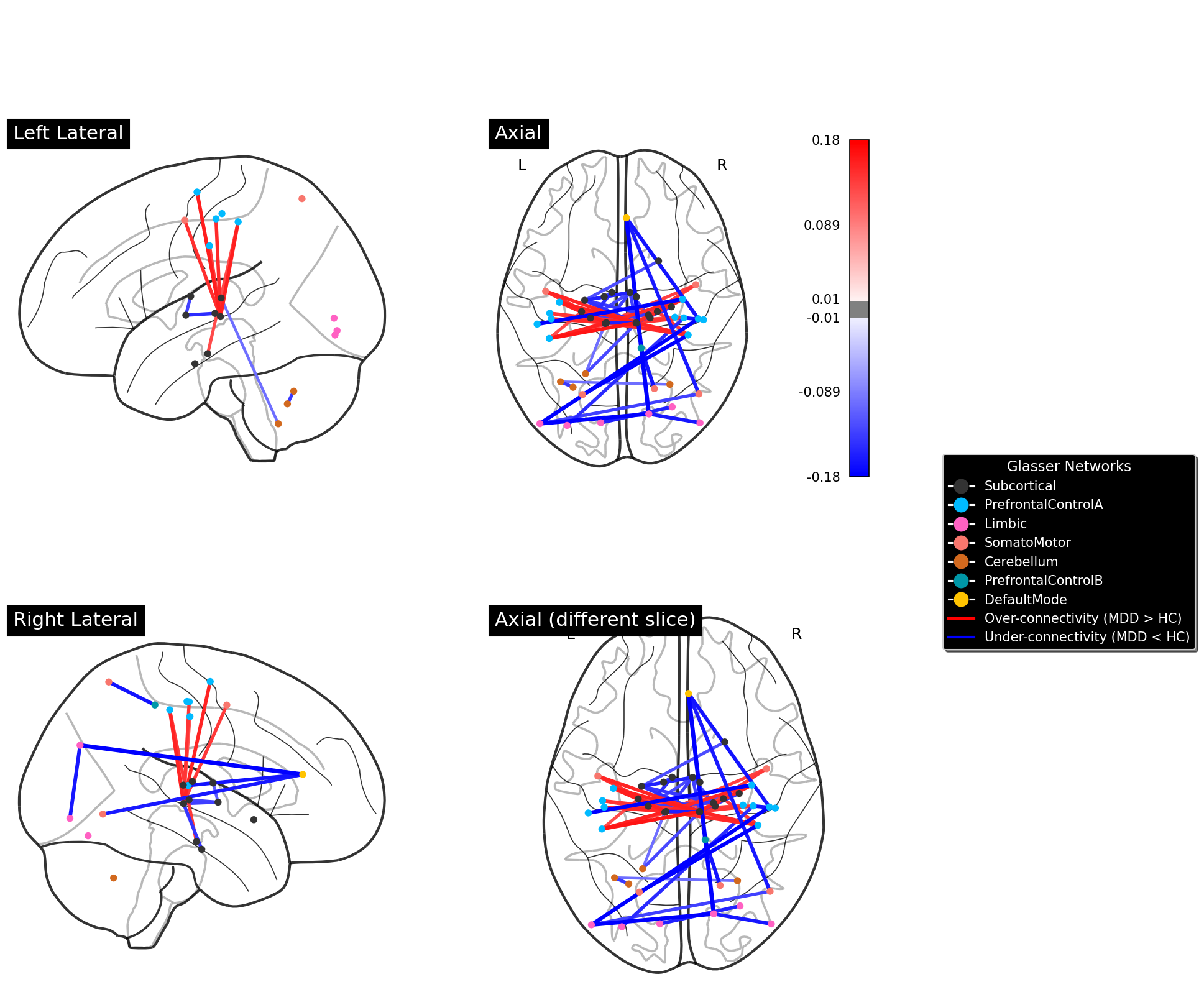
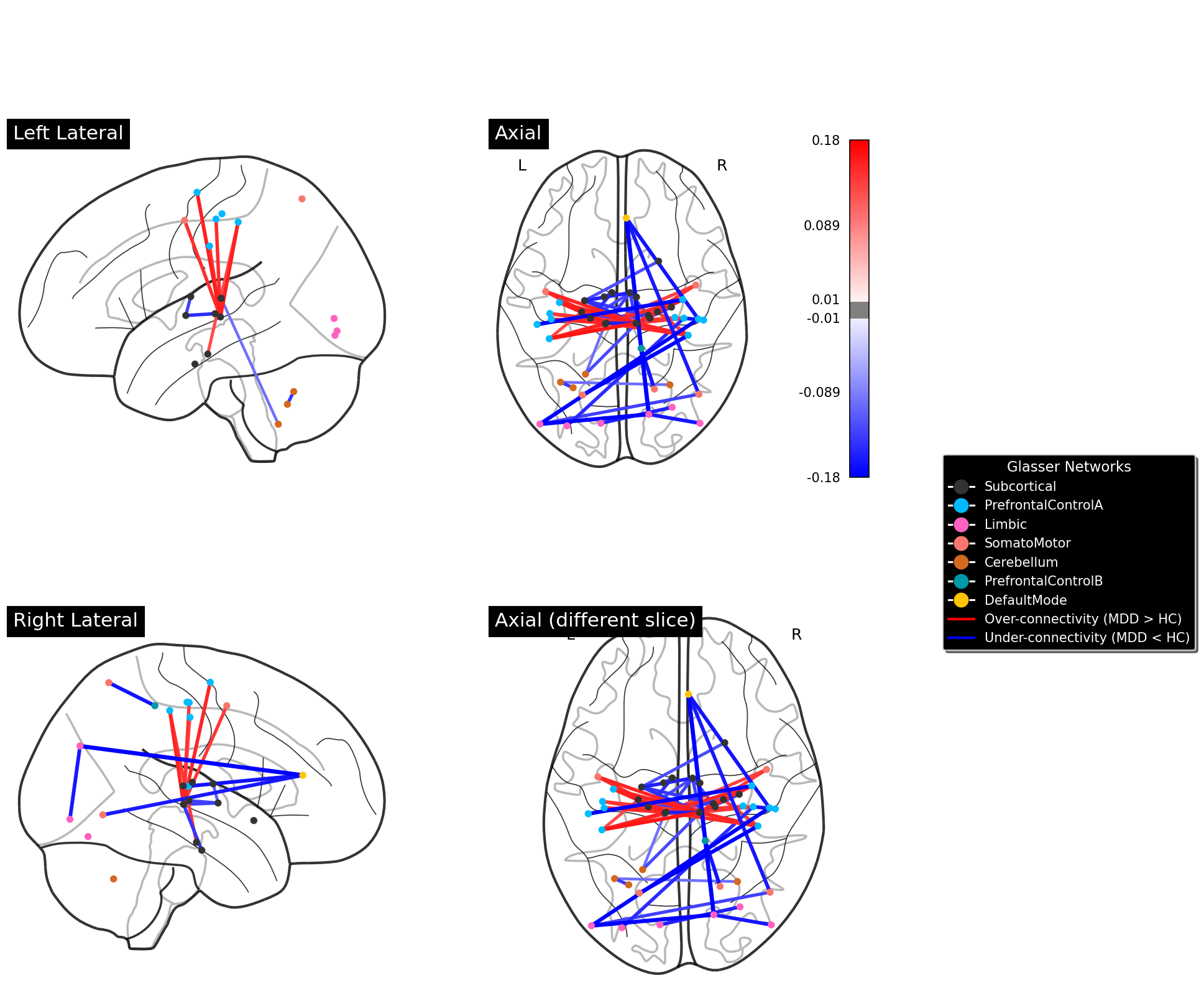
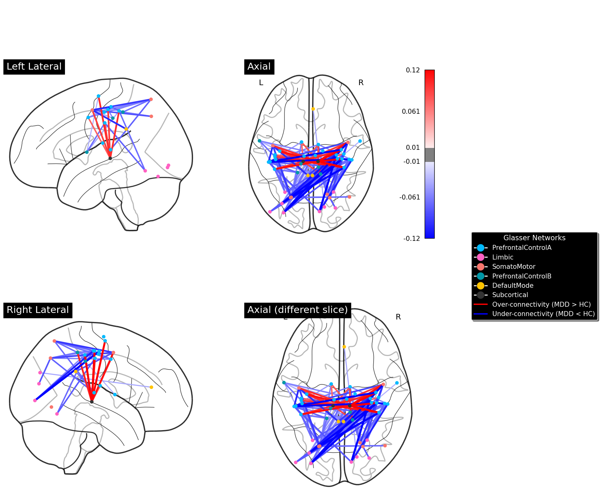
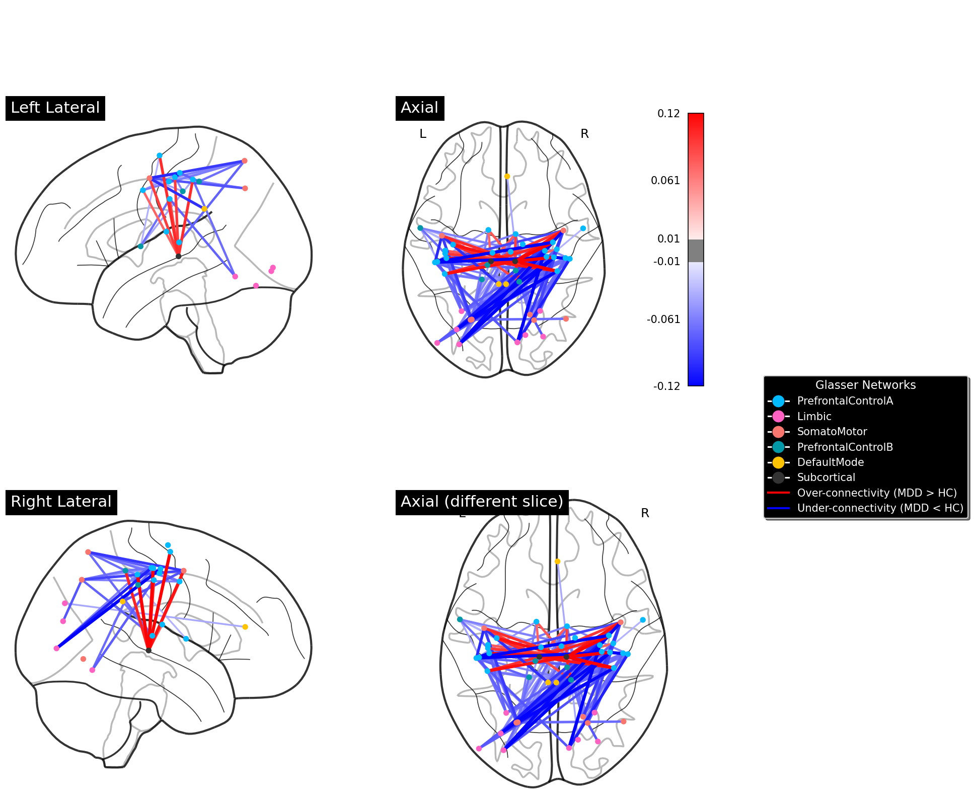
Figure 25: SRPB 100% consensus diagnostic fuzzy FC plot

Figure 26: SRPB original diagnostic FC plot

PCA Feature Selection Stability Results

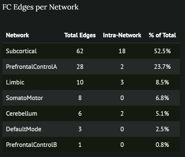
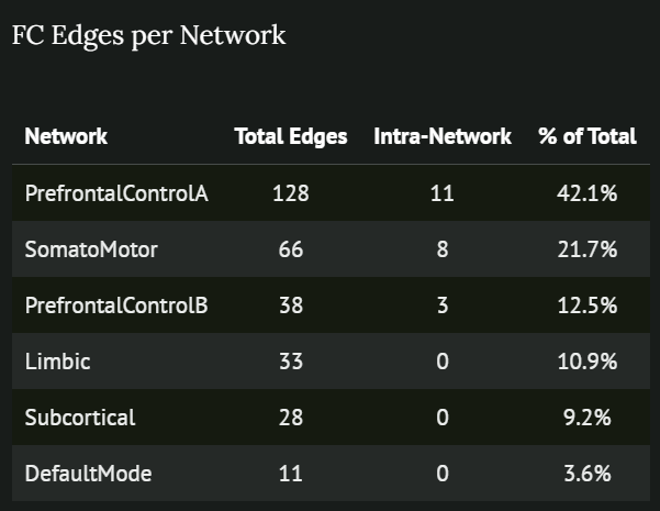
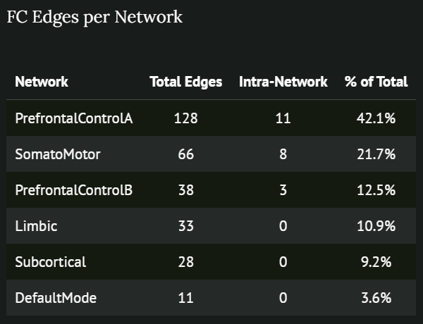
Figure 27: SRPB 100% consensus FC edge per network plot

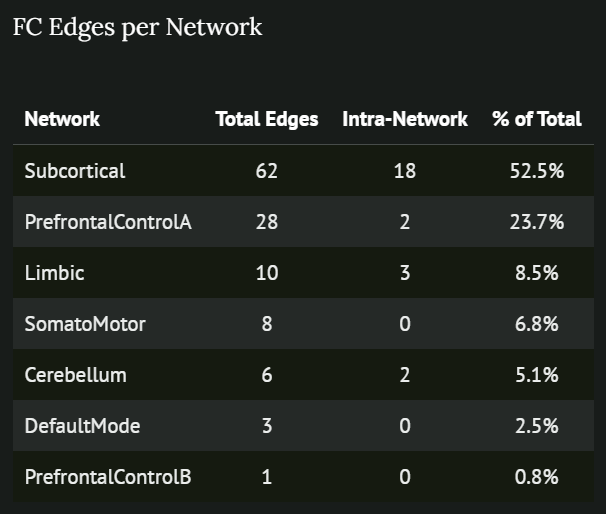
Figure 28: SRPB original FC edge per network plot

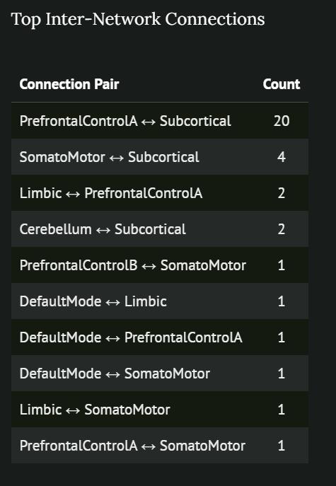
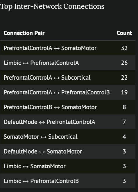
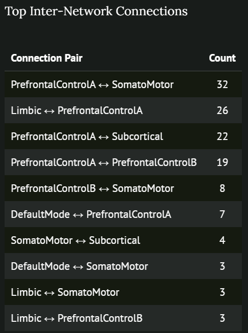
Figure 29: SRPB 100% consensus FC inter connections plot

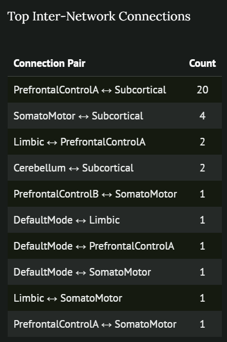
Figure 30: SRPB original FC inter connections plot

PCA Feature Selection Stability Results

Figure 31: BMB fuzzy run 0 diagnostic PC plot

Figure 32: BMB original diagnostic PC plot

Figure 33: BMB 100% consensus diagnostic fuzzy FC plot

Figure 34: BMB original diagnostic FC plot

PCA Feature Selection Stability Results

Figure 35: BMB 100% consensus edge per network plot

Figure 36: BMB original edge per network plot

Figure 37: BMB 100% consensus FC inter connections plot

Figure 38: BMB original FC inter connections plot

Conclusion

The PC selection step of the PCA feature extraction has been improved, and the complete pipeline seems to be very stable now!

It would be interesting to perturb more steps of the FC matrices extraction other than the np.corrcoef.

The subject was very interesting and I’m very grateful to all of you and Prof. Esteban for giving me this opportunity.

I also want to thank Dr. Chatelain for his help on the Fuzzy related things.

Additional Resources

This slide deck is available at this address:
https://olivier.amacker.dev/bachelor-thesis/site/presentations/cbi_presentation.html

Figure 39: Slide deck QR code

References

Alizadeh, Mina, Yohan Chatelain, Gregory Kiar, and Tristan Glatard. 2026. “Numerical Variability of Functional MRI Graph Measures.” bioRxiv. https://doi.org/10.64898/2025.12.22.695524.

Chatelain, Yohan, Andrzej Soko-lowski, Madeleine Sharp, Jean-Baptiste Poline, and Tristan Glatard. 2026. “The Practical Impact of Numerical Variability on Structural MRI Measures of Parkinson’s Disease.” bioRxiv. https://doi.org/10.64898/2026.01.09.698203.

Denis, Christophe, Pablo De Oliveira Castro, and Eric Petit. 2018. “Verificarlo: Checking Floating Point Accuracy Through Monte Carlo Arithmetic.” https://arxiv.org/abs/1509.01347.

Esteban, Oscar, Christopher Markiewicz, Ross Blair, Craig Moodie, Ayse Isik, Asier Erramuzpe, James Kent, et al. 2019. “fMRIPrep: A Robust Preprocessing Pipeline for Functional MRI.” Nature Methods 16 (January). https://doi.org/10.1038/s41592-018-0235-4.

Yamashita, Ayumu, Takashi Itahashi, Yuki Sakai, Masahiro Takamura, Hiroki Togo, Yujiro Yoshihara, Tomohisa Okada, et al. 2026. “Extraction of Robust Functional Connectivity Patterns Across Psychiatric Disorders Using Principal Component Analysis-Based Feature Selection.” Imaging Neuroscience 4 (February): IMAG.a.1121. https://doi.org/10.1162/IMAG.a.1121.

Annex

Here is how the NPVR is calculated in details:

\[ \sigma_{num}^2 = \frac{1}{m} \sum_{j=1}^m \left[ \frac{1}{n-1} \sum_{i=1}^n \left( x_{i,j} - \bar x_{.,j}\right)^2\right] \]

\[ \sigma_{pop}^2 = \frac{1}{n} \sum_{i=1}^n \left[ \frac{1}{m-1} \sum_{j=1}^m \left( x_{i,j} - \bar x_{i,.}\right)^2\right] \]

\[ NPVR = \frac{\sigma_{num}}{\sigma_{pop}} \]

Confounds Used For The Fuzzy FC Matrices Analysis

{
    "confound_columns": [
        "trans_x",
        "trans_y",
        "trans_z",
        "rot_x",
        "rot_y",
        "rot_z",
        "global_signal",
        "csf",
        "white_matter",
        "a_comp_cor_00",
        "a_comp_cor_01",
        "a_comp_cor_02",
        "a_comp_cor_03",
        "a_comp_cor_04",
        "a_comp_cor_05"
    ],
    "filtered_out_confound_columns": [
        "global_signal"
    ]
}